Introduction

SVM was probably the most powerful classic machine learning algorithm before neural network in practice.

Before really dive into SVM, there are several terminologies worth to introduce, one is call hyperplane, it defines as in a p-dimensional space, a hyperplane is a flat affine subspace of dimension p-1 [1], to make it more concrete, in 3-d, the hyperplane is a plane. Whereas, in 2-d, the hyperplane is a line.

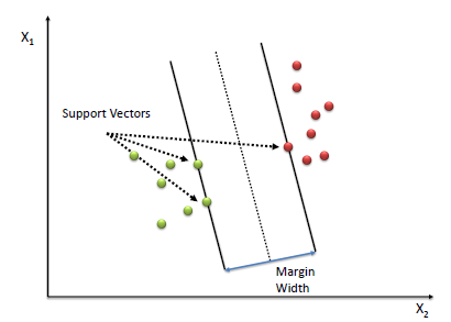
Next concept is called margin, suppose we have a svm plot like following as you can see from the image above, the hyperplane is the dash line in the middle, the margin is the width from the solid line to dash line, we have support vectors to define margin. Which are the closest point to the hyperplane. However, we may not always have such perfect case. Suppose data point are interleaving, we can not find a hyperplane perfectly separate two classes. However, if we can tolerate certain level of misclassifying and find a hyperplane to minimize this error, we call this soft margin.

Maximal margin classifier

I have to give a math definition for later use, to define a hyperplane in math equation \[ \beta_0 + \beta_1X_1 + \beta_2X2 + \cdots + \beta_pX_p = 0 \] if \(p=2\) we have a line, if \(p=3\) we will have a plane. Supposing we have a point in p-dimension that satisfies the equation above, we say that this point is sitting on this plane. If not, this point is either in \[ \beta_0 + \beta_1X_1 + \beta_2X2 + \cdots + \beta_pX_p > 0 \] or \[ \beta_0 + \beta_1X_1 + \beta_2X2 + \cdots + \beta_pX_p < 0 \] we know that the middle dash line is our decision boundary. Therefore, any point lies on the line equal to zero. Otherwise, not greater than or less than zero. Moreover, the larger the value the longer the distance between the point and the line. Therefore, if you only need decide the margin, we do not need all points, we know need three as above which we call it support vectors. This seems like a greate property, since we do not have to calculate many observations.

for people who have used sklearn might notice, the svm classifier in sklearn has a same parameter called C. However, they are opposite each other, the C in sklearn is the penalty term. Which means if you give a big C value, when the classifier misclassifies points, it will get big penalty, in other words, the classifier must make less misclassification to reduce the error or you could say narrowing down the margin and vise versa.

Non-linear decision boundary

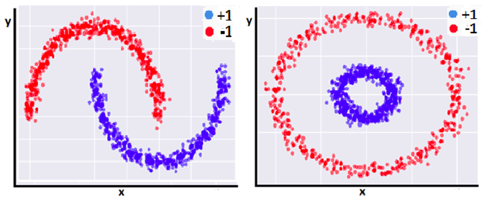
suppose we have dataset like following:

It’s obviousely that we cannot use linear classifier to make the decision boundary any more. However, what if we can transform the original feature space to higher order? we have an similar example like the right side of above image. It has become linearly separable.