Introduction
Linear regression is probably the first topic that every machine learning course will talk. It is simple and often prodivde and adequate and interpretable description of how the inputs affect the output [1]. I will try my best to explain linear regression in a simple way but also with depth insight. For those who scare of math, it is okey just give a glance.
Let’s start from a very simple equation from high school.
\[ y = ax + b \] Here y is outcome or sometimes we will written as \(f(x)\), it is the same thing but written in a different format. a is the slope and b is the intercept. Let’s giving a plot.
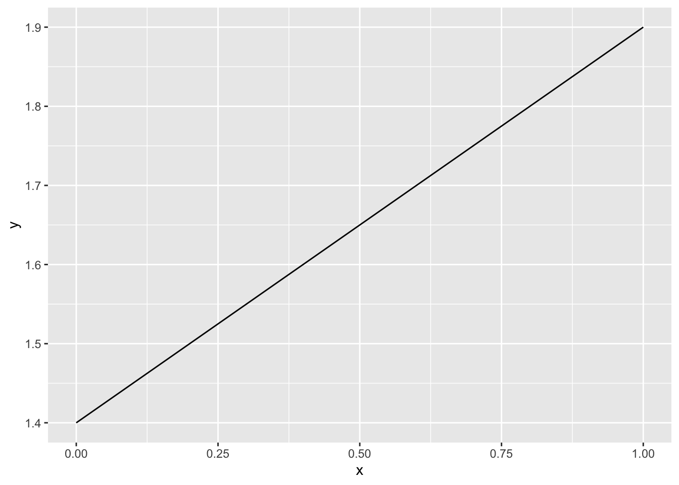 This example is set intercept to 1.4 and slope as 0.5. For this example, we only
have one input (x) and one output (y)
This example is set intercept to 1.4 and slope as 0.5. For this example, we only
have one input (x) and one output (y)
In real world application, we normally have more than one feature. Suppose we have an input vector \(X^T=(X_1, X_2, \dots, X_p)\)
| X | TV | Radio | Newspaper | Sales |
|---|---|---|---|---|
| 1 | 230.1 | 37.8 | 69.2 | 22.1 |
| 2 | 44.5 | 39.3 | 45.1 | 10.4 |
| 3 | 17.2 | 45.9 | 69.3 | 9.3 |
| 4 | 151.5 | 41.3 | 58.5 | 18.5 |
| 5 | 180.8 | 10.8 | 58.4 | 12.9 |
Here the input features we could think as X1=TV, X2=Radio and X3=Newspaper. and the y is Sales
We have a simple model for multiple features
\[ f(X)=\beta_{0}+\sum_{j=1}^{p} X_{j} \beta_{j} \]
Let’s plot a regression model for iris dataset to see what exactly going on.
ggplot(df, aes(TV, Sales)) +
  geom_point() +
  geom_smooth(method = 'lm', formula = y~x)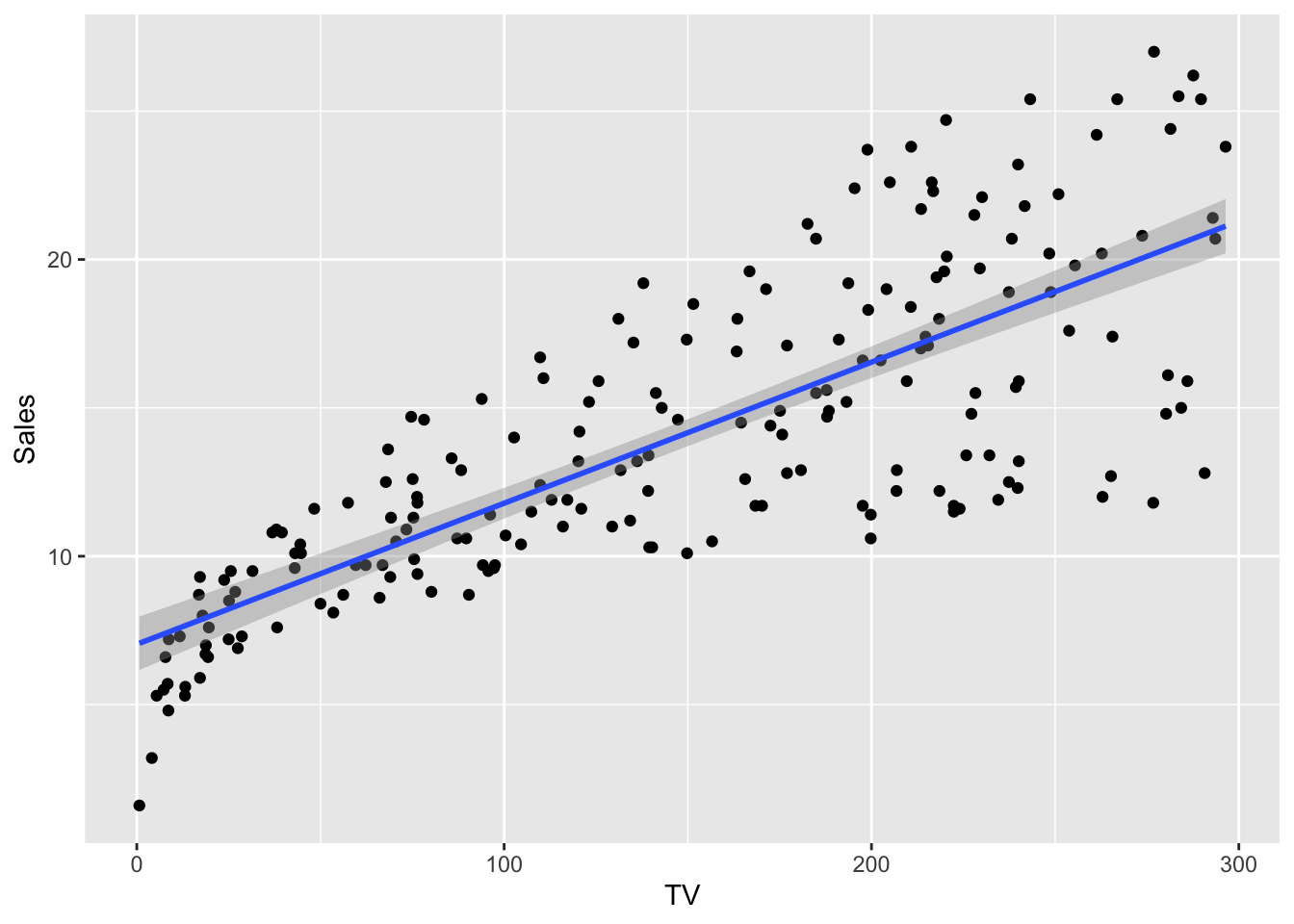
What we like to do is reduce the residuals.

png
So finally, what we want to do is just minimize the residual sum of squares, which is the equation following: \[ \begin{aligned} \operatorname{RSS}(\beta) &=\sum_{i=1}^{N}\left(y_{i}-f\left(x_{i}\right)\right)^{2} \\ &=\sum_{i=1}^{N}\left(y_{i}-\beta_{0}-\sum_{j=1}^{p} x_{i j} \beta_{j}\right)^{2} \end{aligned} \]
To make the formula clear little bit. We could using vectorization or vector notation to represent it.
\[ \operatorname{RSS}(\beta)=(\mathbf{y}-\mathbf{X} \beta)^{T}(\mathbf{y}-\mathbf{X} \beta) \]
let’s take the derivative respect to \(\beta\). \[ \frac{\partial \mathrm{RSS}}{\partial \beta}=-2 \mathbf{X}^{T}(\mathbf{y}-\mathbf{X} \beta) \]
Because, if we check the RSS equation above it is a quadratic function. Therefore, this equation is always having a global minimal value. Let’s just set the derivative equal zero, then find what the \(\beta\) is.
\[ \begin{aligned} &-2 \mathbf{X}^{T}(\mathbf{y}-\mathbf{X} \beta)=0 \\ &\mathbf{X}^{T}(\mathbf{y}-\mathbf{X} \beta)=0 \quad (1)\\ &\mathbf{X}^{T}\mathbf{y}-\mathbf{X}^{T}\mathbf{X} \beta=0 \quad (2) \\ &\mathbf{X}^{T}\mathbf{y}=\mathbf{X}^{T}\mathbf{X} \beta \quad(3)\\ &(\mathbf{X}^{T}\mathbf{X})^{-1}\mathbf{X}^{T}\mathbf{y}=(\mathbf{X}^{T}\mathbf{X})^{-1}\mathbf{X}^{T}\mathbf{X} \beta \quad (4)\\ &(\mathbf{X}^{T}\mathbf{X})^{-1}\mathbf{X}^{T}\mathbf{y} = \beta \quad (5) \end{aligned} \]
Let’s break it down, the first step we just divide both side by -2, hence we can eliminate the constant. Second step we just apply distribution rule, the third one is to make the equation equal, we just move \(-X^tX\beta\) to the right side. Step 4 is just using a little trick to make \(X^TX\) to an identity matrix by multiply \((X^TX)^{-1}\), finally, we get \(\beta\).
It is obviously that if we multiply \(X\) to the \(\beta\) we can calculate the estimated \(\hat{y}\) value
Case study
It is important for an analyst to understand the output of a linear model. It is not just blindly using some packages without thinking. Here I take an example from book An Introduction to Statistical Learning [2].
Let’s start from single variable linear regression model, then try to give
a short explanation to the output. Here we use Boosten dataset from R package
of MASS, this dataset records 506 neighborhoods around Boosten, there are several
feature columns, like crim indicates per capita crime rate by town, rm means
the average number of rooms per dwelling and ptratia means pupil-teacher ratio
by town.
Here we use feature lstat (lower status of the population) to predict
medv(median value of owner-occupied homes in $1000).
lm.fit <- lm(medv ~ lstat, data = MASS::Boston)
summary(lm.fit)
##
## Call:
## lm(formula = medv ~ lstat, data = MASS::Boston)
##
## Residuals:
## Min 1Q Median 3Q Max
## -15.168 -3.990 -1.318 2.034 24.500
##
## Coefficients:
## Estimate Std. Error t value Pr(>|t|)
## (Intercept) 34.55384 0.56263 61.41 <2e-16 ***
## lstat -0.95005 0.03873 -24.53 <2e-16 ***
## ---
## Signif. codes: 0 '***' 0.001 '**' 0.01 '*' 0.05 '.' 0.1 ' ' 1
##
## Residual standard error: 6.216 on 504 degrees of freedom
## Multiple R-squared: 0.5441, Adjusted R-squared: 0.5432
## F-statistic: 601.6 on 1 and 504 DF, p-value: < 2.2e-16Let’s interpret the summary one by one. The first is the call field, it is just simply the formula of this model, nothing special. Next one is the statistical summary for residuals, actually we can use box plot to show it more concretely.
ggplot(data.frame(resi = residuals(lm.fit)), aes(x = "", y = resi )) +
  geom_boxplot()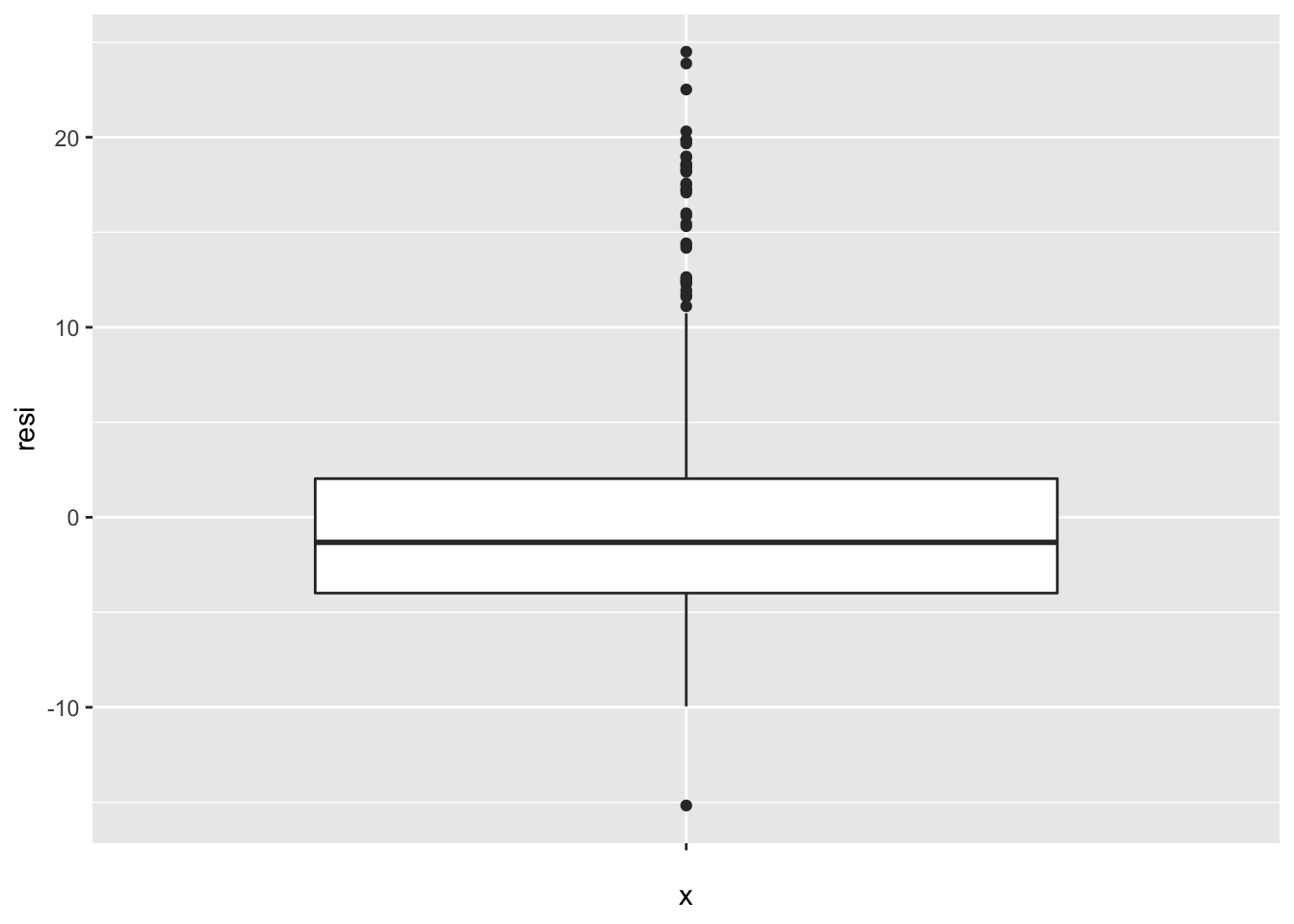
As we can see, the plot above matches the summary. The middle thicker horizontal line is the median (-1.318) in the summary, and the line above and below the median line is the first quantile (1Q) and third quantile (3Q). The points on the top and bottom is the min and max value.
The next important field is Coefficients, by observing this field, we can find the how predict variables affect the response variable, this is why linear regression model is an interpretable model.
If you recall from the beginning of this blog, there is a formula \(y = ax + b\)
here the intercept is 34.55384, we can think this value is as \(b\) in the formula
and \(a\) is lstat which is -0.95005. Just by these information, we could know
that lstat and medv is negatively related, which means when lstat increase
1 unit, medv will decrease -0.95005. Std. Error here can be use to calculate
the confidence interval and t value is used to calculate p-value. Therefore,
if we really want to know the confidence interval for coefficients, we can use
function confint in R.
confint(lm.fit)## 2.5 % 97.5 %
## (Intercept) 33.448457 35.6592247
## lstat -1.026148 -0.8739505The confidence interval just like asking people to guess something, suppose ask a veteran mechanics what is the probability that a certain engine will be broken, he will give his experienced guess but with amount of uncertainty, but if you ask an amateur, he will also give his guess but with a more large range of uncertainty.
Just by knowing the confidence interval you could know that if a coefficient significant of not. When there is a 0 appears between the confidence interval you could confirm that this coefficient is not significant, because there may have a chance the coefficient becomes 0. Which makes that input feature no meaning at all.
After building the model, we can use this model to predict new coming data
lm.pred <- predict(lm.fit, data.frame(lstat=(c(5,10,15))), interval = "confidence")
lm.pred
## fit lwr upr
## 1 29.80359 29.00741 30.59978
## 2 25.05335 24.47413 25.63256
## 3 20.30310 19.73159 20.87461the test data is confirming our interpretation above, as lstat increasing
medv decreasing. Notice, here we use a special parameter, interval=“confidence”.
this parameter will give the prediction around the mean of the prediction. To interpret the result above, with 10 lstat on average the value for medv is
between 24.47 and 25.63.
We can set the parameter inverval as “prediction” as well. However, this prediction only give the prediction interval around a single value. This setting is highly rely on residuals are normally distributed. I will give the methods how to test the normality of residuals in the caveat section.
Caveats
Linear regression model has its limitation or more precisely saying it has assumption For example, as the name indicates, there must be a linear relationship between predict variables and response variable, because the solution will either line plane or hyperplane which is not curvy. I list several assumptions regard to linear regression.
- residuals are roughly normally distributed
- residuals are independent
- linear relation between features and output
- no or little multicollinearity
- homoscedasticity (residuals agains fitted value should keep constant)
- sensitive to outliers
There are several ways to test the assumptions
residual normality
By checking residuals normality, we can use Q-Q plot,
lm.fit <- lm(medv ~ rm + lstat + crim + dis, data = Boston)
ggqqplot(residuals(lm.fit))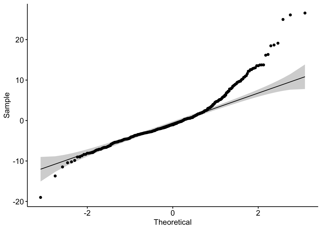
How to interpret this plot? Suppose the residuals are following a normal distribution, the points above should be roughly located around the slope line and should be with inside the 95% confidence curvy dashed line.
In a algorithmic way to check, we could utilize Shapiro-Wilk test [3].
shapiro.test(residuals(lm.fit))##
## Shapiro-Wilk normality test
##
## data: residuals(lm.fit)
## W = 0.91081, p-value < 2.2e-16As the result p-value indicates (<0.05). We can reject the null hypothesis (normally distributed). Therefore, the residuals is not normally distributed. Here we can see, it is important to do both visual and algorithmic test, the plot above shows us a roughly normal distributed data. However, the test indicates this is not a normally distributed data.
residuals independency
By plotting the residuals along with the order of \(Y_i\) we can measure the residuals independency.
plot(sequence(nrow(Boston)), residuals(lm.fit))
abline(h=0, col='red')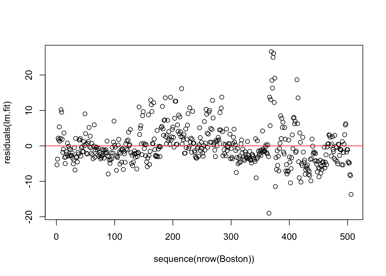
Independent residuals should be located around 0 and randomly scattered.
linearity
linearity is just checking if the predict variables (input X) has the linear relation between the response variable. After all, we use linear regression to create model, if there is no linear relation we have to use other non-linear model.
crPlots(lm(medv ~ rm + lstat + crim + dis, data = Boston))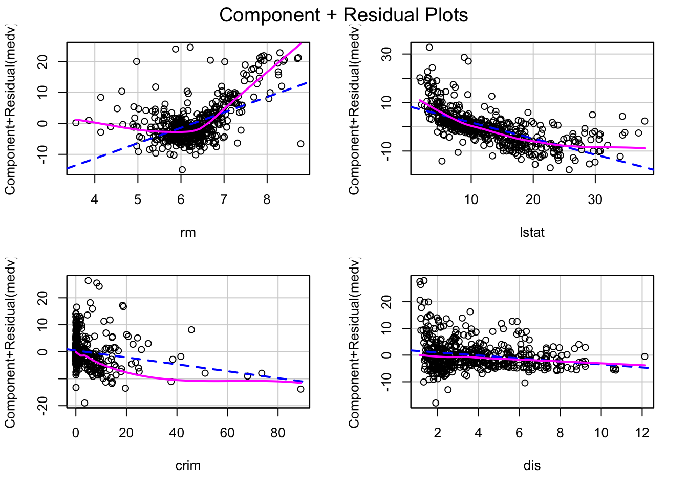
what we most case is if there is any pattern inside the plot
summary(gvlma::gvlma(x = lm.fit))##
## Call:
## lm(formula = medv ~ rm + lstat + crim + dis, data = Boston)
##
## Residuals:
## Min 1Q Median 3Q Max
## -19.006 -3.099 -1.047 1.885 26.571
##
## Coefficients:
## Estimate Std. Error t value Pr(>|t|)
## (Intercept) 2.23065 3.32214 0.671 0.502
## rm 4.97649 0.43885 11.340 < 2e-16 ***
## lstat -0.66174 0.05101 -12.974 < 2e-16 ***
## crim -0.12810 0.03209 -3.992 7.53e-05 ***
## dis -0.56321 0.13542 -4.159 3.76e-05 ***
## ---
## Signif. codes: 0 '***' 0.001 '**' 0.01 '*' 0.05 '.' 0.1 ' ' 1
##
## Residual standard error: 5.403 on 501 degrees of freedom
## Multiple R-squared: 0.6577, Adjusted R-squared: 0.6549
## F-statistic: 240.6 on 4 and 501 DF, p-value: < 2.2e-16
##
##
## ASSESSMENT OF THE LINEAR MODEL ASSUMPTIONS
## USING THE GLOBAL TEST ON 4 DEGREES-OF-FREEDOM:
## Level of Significance = 0.05
##
## Call:
## gvlma::gvlma(x = lm.fit)
##
## Value p-value Decision
## Global Stat 638.73 0.000e+00 Assumptions NOT satisfied!
## Skewness 143.63 0.000e+00 Assumptions NOT satisfied!
## Kurtosis 289.67 0.000e+00 Assumptions NOT satisfied!
## Link Function 175.67 0.000e+00 Assumptions NOT satisfied!
## Heteroscedasticity 29.76 4.902e-08 Assumptions NOT satisfied!hemoscedasticity
For checking hemoscedasticity. Which means the variance of residuals should be constant, see the plot below.
par(mfrow=c(2,2))
plot(lm.fit, pch = 16, cex = 0.5)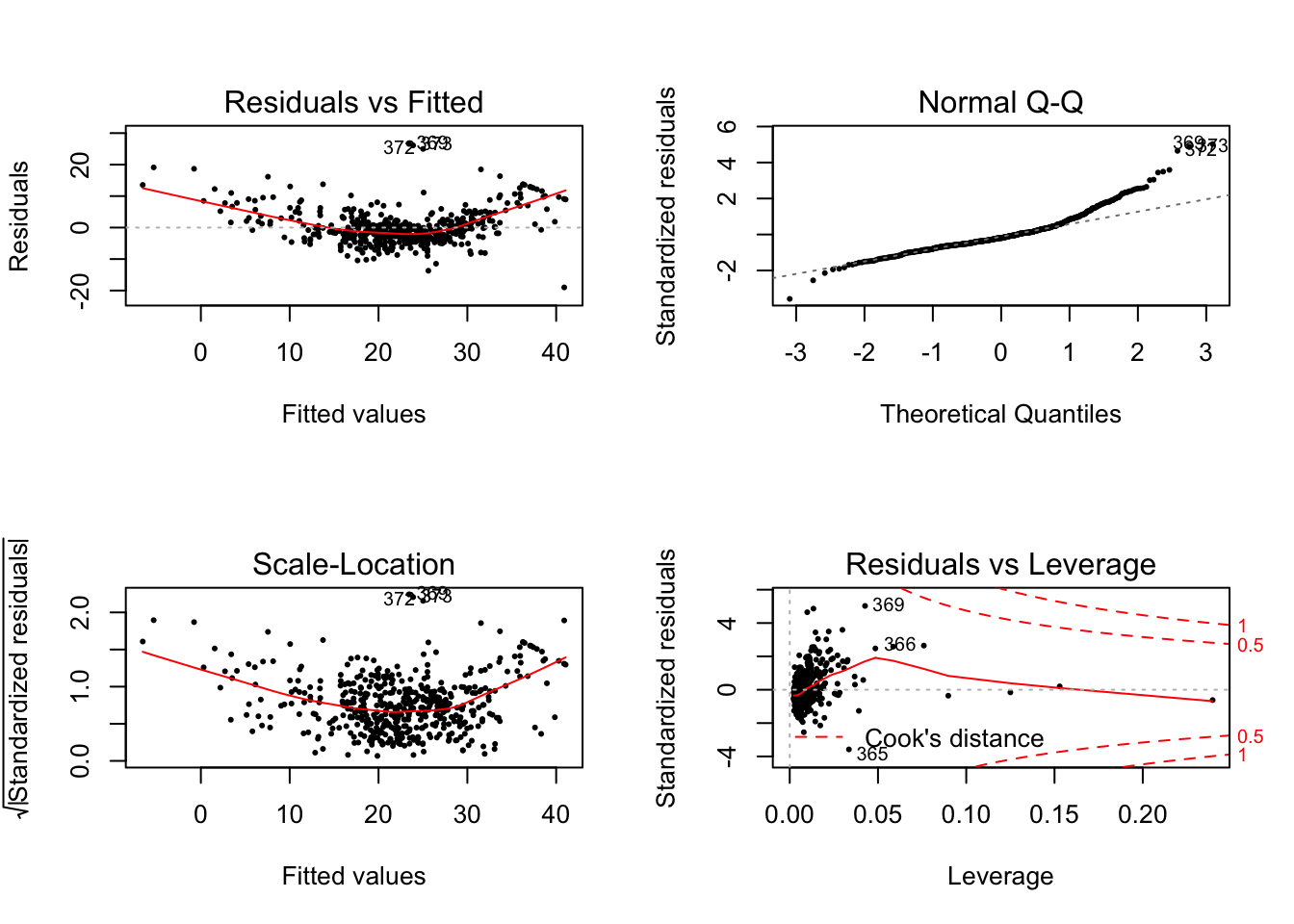 We are intereted in the left side two plots. To express homoscedasticity in a plot,
it would look like a roughly flat line with random points around it. However, in
our case here [4]. We could find the red line is curvy and the
points have a growth trend from left to right.
We are intereted in the left side two plots. To express homoscedasticity in a plot,
it would look like a roughly flat line with random points around it. However, in
our case here [4]. We could find the red line is curvy and the
points have a growth trend from left to right.
If you think visualization is not enough to determine if a model is hemoscedasticity, There are several algorithmic ways to test as well.
car::ncvTest(lm.fit)## Non-constant Variance Score Test
## Variance formula: ~ fitted.values
## Chisquare = 0.4130551, Df = 1, p = 0.52042By checking the p-value, we could see that is significant (<0.05) enough to reject the null hypothesis (variance is constant).
outliers
Because we use RSS to estimate the accuracy, it is obviousely that outliers will highly influence the RSS. Which makes the wrong interpretation to the model.
A data point has high leverage, if it has extreme predictor x values [5]. Let’s using Residuals vs Leverage plot
par(mfrow=c(1,2))
plot(lm.fit, 4)
plot(lm.fit, 5, pch = 16, cex = 1)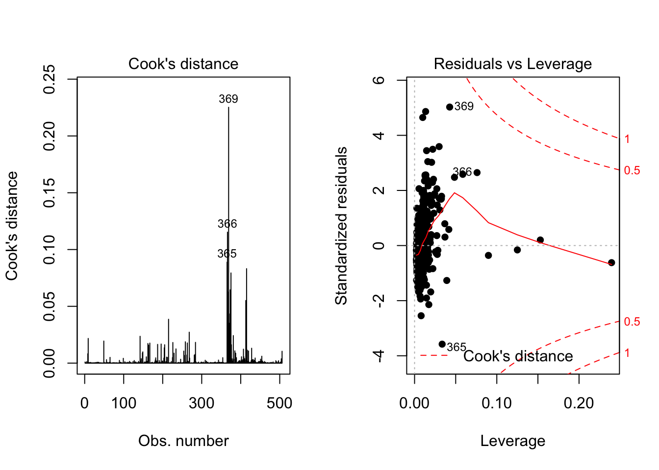
The plot above shows that #23, #49 and #39 are influenced points. Among those three points, #23 and #49 are close to 3 standard deviation. Which is more influential than #39. However, are these outliers really influence the result of the regression analysis? Here we need one metric called Cook’s distance to check if data points really influential.
A rule of thumb is that an observation Cook’s distance exceeds \(4/(n-p-1)\), where \(n\) is the number of observations and \(p\) is the predictor variables. Thus, we can calculate Cook’s distance for this model, which is 4/(50-1-1) = 0.08. We can add a horizontal line to the Cook’s distance plot
olsrr::ols_plot_cooksd_bar(lm.fit)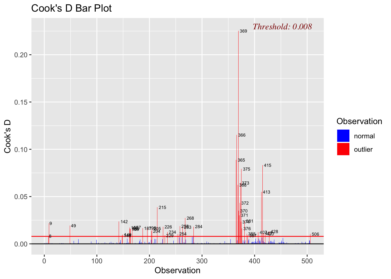
As we can see above, data point #23 and #49 are really influence the result of linear regression analysis.
References
1. The elements of statistical learning.
Friedman J, Hastie T, Tibshirani R.
Springer series in statistics New York; 2001.
2. An introduction to statistical learning.
James G, Witten D, Hastie T, Tibshirani R.
Springer; 2013.
3. Shapiro-Wilk Test [Internet].
Lohninger H.
2012;Available from: http://www.statistics4u.info/fundstat_eng/ee_shapiro_wilk_test.html
4. How to detect heteroscedasticity and rectify it? [Internet].R-bloggers2016;Available from: https://www.r-bloggers.com/how-to-detect-heteroscedasticity-and-rectify-it
5. Linear Regression Assumptions and Diagnostics in R: Essentials - Articles - STHDA [Internet].2019;Available from: http://www.sthda.com/english/articles/39-regression-model-diagnostics/161-linear-regression-assumptions-and-diagnostics-in-r-essentials