Introduction
Although nowadays deep learning is gaining more attention than classic machine learning methods, classic machine learning algorithm is still have its advantage than deep learning cannot beat, like simplicity and interpretability. Among classic machine learning algorithm, decision tree or more accurate its variation like random forest or bagging is widely used in industry. The beauty of decision tree is that it closes to human making decision.
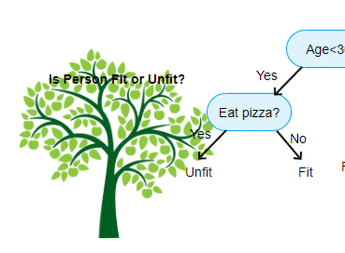
There are several terms worth to explain in front. Here is an image to help me
to illustrate it

Normally, a tabular data is binary splitting into the tree like a bove, we are choosing a feature (colume) to split the data (row), the decision node we call it internal node, then we recursively split the tree until we reach certain threshold for example only two observations in the terminal node, terminal node is the end of a tree, we call it leaf node as well.
As you can see above, the first internal node probably the most important factor among other nodes, because based on this decision we decide where to go. Therefore, this nature makes decision easy to interpret. Moreover, each terminal node is actually divided into rectangle as you can see from the left on the image above.
So is decision tree able to be used in regression and classification tasks as other machine learning algorithms?
Regression tree
Regression tree can be used in a regression task like linear regression, so how does regression do a prediction? A regression tree predicted value is the mean response of the training observations [1]. To make it simple, when we built our decision tree, the predicted value is just the average value in each terminal nodes or each rectangle. The way to decide the splitting value is by minimize the mean value with each observations in each rectangle. \[ \sum_{j=1}^J\sum_{i\in R_j} (y_i-\hat{y}_{R_j})^2 \] Here, \(R_j\) is the rectangle or terminal node. What we have to do is just minimize the total error. When we doing a prediction, we just give a training observation based on decision we find the rectangle it belongs to, then we find the mean value inside that region. So how does a classification task can be done by decision tree?
Classification tree
Classification tree is nothing special than a regression tree, only difference is the error measurement. For classfication problems, we don’t have quantitative ground truth, instead we have qualitative value. Therefore, one measure called Gini index was introduced, Gini index is defined by \[ G = \sum_{k=1}^K \hat{p}_{mk}(1-\hat{p}_{mk}) \] this is a measure of total variance across K classes, Where \(\hat{p}_{mk}\) is the proportion of observations in the mth region (rectangle) for kth class. Gini index measures the purity of nodes, or call it impurity [2] why? as you can see the smaller the value the more a node from single class. in other words, this node is not impure. Which more close to human intuition. Another measure is called entropy, it is defined as \[ E = -\sum_{k=1}^K \hat{p}_{mk}log_2(\hat{p}_{mk}) \] as you can see, this measurement is close to Gini index measurement. Here I created an artificial dataset to demostrate how to use entropy. Supposing we have 2-class dataset like following
| x1 | x2 | y |
|---|---|---|
| 1.5 | 2.3 | 0 |
| 1.8 | 3.2 | 0 |
| 1.3 | 3.3 | 0 |
| 2.1 | 3.1 | 1 |
| 2.3 | 3.4 | 1 |
| 2.8 | 4.0 | 1 |
if we split the tree based on \(x1 <= 1.8\), the node on the left will purely belongs to class 0, where the right node will all belongs to class 1. This is a better choice against \(x2\). Why? because the entropy for the left node is 0, and so as right node. Whereas, if we choose \(x2 <= 3\) as our splitting node, we will have entropy for left node is 0, but for right node we have entropy \((-0.4*log(0.6)) + (-0.6*log(0.6)) = 0.97\). Which compared to splitting by \(x1\) is less optimal.
Here is a plot to show the differences for different measurement methods [3]
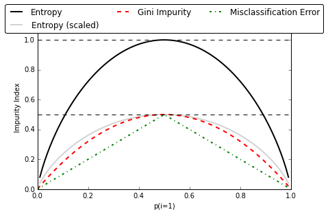
measure
Pruning
when you don’t specify the max depth for decision tree, decision tree will lead to overfitting. Pruning is for prevent overfitting, there are two strategies to prun a tree, one is called prepruning, which stop earlier when training a tree. Whereas, another is called postpruning, which allows the tree grow freely then pruning the tree. Each has its one advantage over other, for example prepruning will training fast, whereas, postpruning usually has a good accuracy over prepruning.
Pros, Cons
- trees are easy to explain to people (+)
- trees can be displayed graphically (+)
- trees can easily handle qualitative variable without creating dummy variable (+)
- no need to center or scale data (+)
- no as accurate as other regression and classification methods (-)
However, by adding more decision trees, the power of decision trees emerge, one representative algorithm is random forest.
Random Forest
random foreset is an ensemble learning algorithm, as the name shows, it consists many decision trees, it also utilizes a statistical method called bootstrap, bootstrap is a way to sample data from a limited datasets, so that we can have enough dataset to train. random forest is similar like bagging algorithm the difference between bagging algorithm is that random forest using fewer predictor variable (feature) to training. Which will help reduce the correlation between predictor variables. One advantage of random forest is that even add more decision trees, there will not lead to overfitting. There are other algorithms based on decision tree, like Adaboosting, XGBoosting, CART, etc.
Tips
Here are some tips from practice [4] regard to sklearn.
- consider performing dimension reduction before training model
- using depth=3 as an starting tree to get a feel how the tree look like
- use max_depth to control size of the tree to avoid overfitting
- when using random forest, choose the training feature as sqrt(total feature)
- when using boosting, a typical learning rate \(\lambda=(0.01,0.001)\) will be a good start
demo for decision tree ### References
1. An Introduction to Statistical Learning [Internet].
James G, Witten D, Hastie T, Tibshirani R.
New York, NY: Springer New York; 2013 [cited 2019 Nov 8]. Available from: http://link.springer.com/10.1007/978-1-4614-7138-7
2. Introduction to machine learning.
Alpaydin E.
2nd ed. Cambridge, Mass: MIT Press; 2010.
3. Decision trees: An overview and their use in medicine.
Podgorelec V, Kokol P, Stiglic B, Rozman I.
Journal of medical systems 2002;26(5):445–63.
4. The online teaching survival guide: Simple and practical pedagogical tips.
Boettcher JV, Conrad R-M.
John Wiley & Sons; 2016.